What do I study?

Over the years, friends, family, and strangers have asked me if I can explain the math that I do. This is tricky; because math is so cumulative, even professional mathematicians usually can’t understand each other’s work very well unless they work in the same field. (This has the advantage of making it difficult to talk about work at parties.) This series is my attempt to share the stuff I think about and why I think it’s so fun.

My area of math is called homotopy theory. Historically, this grew out of topology, which is a form of geometry. Nowadays, it’s increasingly viewed as foundational to math itself, so it interacts with a lot of other fields. In particular, I’m very interested in how it interacts with a subject called arithmetic geometry, which tries to incorporate things like prime numbers into geometry. The field is in a bit of a golden age right now: major papers are being posted nearly every month, and decades-old problems are falling one after another.

What I mainly do is study prismatic cohomology (a hot new thing in arithmetic geometry) from the perspective of equivariant homotopy theory. Equivariant means having to do with symmetry—in this case the rotational symmetry of a circle.

I’ll explain all these fancy words over the course of many posts! A hyper-condensed overview is at the end of this post.

Homotopy theory has a very theoretical side and a heavily computational side; I started out more on the theory side, but now lean more towards calculations. I often make interactive widgets and pretty pictures to help myself understand what I’m doing; pictures are maybe a good thing to organize this series around. My first goal is to explain what’s going on in the following diagram:

Later, I’ll talk about this one:

and maybe eventually these guys:

A rapid overview

Let’s start by thinking about how we represent points on a shape:

Source

We can represent a point on the blue curve by a number between 0 and 1 (between 0% and 100% along the curve, starting from the left). This is the same way we’d represent points on a straight line segment. We can almost do the same thing on the purple star, but now 0% and 100% represent the same point. This is similar to how $0^\circ,$ $360^\circ,$ $720^\circ,$ etc. all correspond to the same point on the circle.

Topology is the study of “how data gets represented”. The blue curve is topologically equivalent to a straight line, and the purple curve is topologically equivalent to a circle. Topology is also often described as “rubber-band geometry”: topology considers two shapes to be the same if each can be transformed into the other by twisting or bending, but no cutting or tearing.

However, the difference between the straight line and the circle is very important. To some extent, “every problem that can be described using numbers, we can solve, and there’s a unique solution”. (This is extremely vague, but I have precise statements in mind.) But suppose the solution involves dividing by $3$. Well, $0/3$ is just $0,$ but $0^\circ/3$ is $\{0^\circ,120^\circ,240^\circ\}.$ When the basic operations we do on numbers are unavailable, or behave differently than usual, we’re no longer able to “solve every problem”.

Homotopy theory goes a step further than topology and adds “inflating and deflating” to the list of operations that “don’t change a shape”. We can shrink a straight line down to a single point (the most trivial shape there is), so these are homotopically equivalent (but not topologically). We can build a circle by taking a straight line and gluing the ends together. When we pass from topology to homotopy, we “delete” the straight line, so the gluing is the only information that’s left. I like to think about this as: we understand numbers pretty well, so we want to ignore those and just focus on the “redundancies” or “wrinkles” in the representation of data.

Cohomology is a quantitative way to describe these “wrinkles” or “redundancies”. In its crudest form, cohomology associates a sequence of numbers (called Betti numbers) to every shape. Here are some examples:

(The two shapes above the $2,\,4$ are considered a single shape; the $2$ means there are two pieces, or connected components. Also, $2,\,4$ is really short for $2,\,4,\,0,\,0,\,0,\,\dotsc$)

There are many different cohomology theories that offer different interpretations of what these numbers mean, and also provide richer information beyond these numbers.

• from the perspective of singular cohomology, these numbers are counting the number of (higher-dimensional) “holes” or “loops” in a shape.

• de Rham cohomology is based on calculus¹. Calculus is about change: e.g. velocity as the rate of change of position, or acceleration as the rate of change of velocity. Although $0^\circ$ and $360^\circ$ represent the same point on a circle, an angular velocity of $360^\circ\text{ / sec}$ is very different from an angular velocity of $0^\circ\text{ / sec}$. So de Rham cohomology sees a numeric quantity (angular velocity) that looks like the rate of change of some other quantity (angle), but the original quantity is “missing”.

If you kind of already know what your shape looks like, you can calculate its cohomology using any cohomology theory. But what if someone just hands you some random equations? De Rham cohomology is fairly easy to calculate “mechanically”—we can program computers to do calculus. But singular cohomology is very abstract, and literally impossible to calculate directly for anything beyond discrete points.

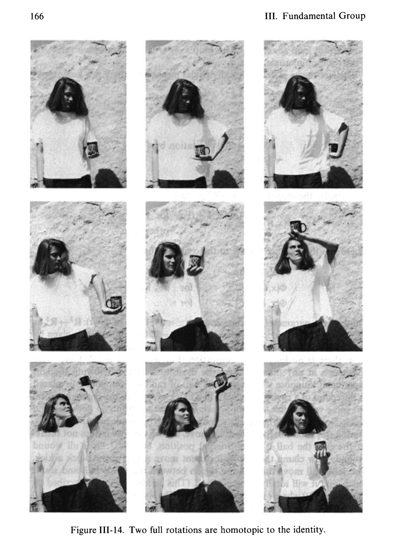
Despite this, singular cohomology has some advantages over de Rham cohomology. Think about the distinction between a line (through the origin) and a direction: you can travel in two directions on every line. This “2:1 redundancy” shows up in many places: it’s responsible for the “plate trick” seen below, as well as the phenomenon of gimbal lock. Gimbal lock causes problems in aviation and 3d graphics, necessitating the use of quaternions for doing rotations. (Rotations in 3d space are (non-obviously) topologically equivalent to lines through the origin in 4d space; unit quaternions are directions in 4d space.)

Taken from Bredon, Topology and Geometry.

Hopefully this convinces you that understanding “2:1” redundancies is important. Unfortunately, de Rham cohomology can only detect “∞:1” redundancies; singular cohomology can detect “finite:1” redundancies, but is much harder to compute. Prismatic cohomology is a fancier version of de Rham cohomology, based on a fancier version of calculus, which is able to detect “finite:1” redundancies, while remaining fairly computable.

The circle (infinitely many angles corresponding to the same point) is the simplest example of cohomology. It is also the universal example: if you think hard enough about the circle, you can deduce the entire theory of de Rham cohomology. (I don’t know why this should be true, or if this is even a good way of thinking about it.) In particular, the rotational symmetries of the circle play a central role in prismatic cohomology.

What I mainly do these days is think about prismatic cohomology from the perspective of these rotational symmetries. There are many other perspectives; this one is historically the first, but the subsequent ones that were discovered are much simpler for most purposes, so this one has been neglected. However, I’ve shown that it illuminates some of the more advanced aspects of the theory.

My main project right now is trying to generalize prismatic cohomology to accommodate other kinds of symmetry. Circles also have reflectional symmetry, in addition to rotational. It’s slightly harder to get “even:1” information out of prismatic cohomology than “odd:1”, and it’s thought that incorporating the reflectional symmetries might explain this. There are several people working on this, from different perspectives than mine, and I’m trying to understand how my approach compares to theirs.

I’m also interested in plugging in completely different kinds of symmetry, like that of a triangle or square. It’s less clear what this would be useful for.

1. I mean differential calculus here, which is about instantaneous rates of change. There’s also integral calculus which is about the reverse: accumulated change over time. In cohomology land, the connection between differential and integral calculus (the fundamental theorem of calculus) translates to the fact that singular and de Rham cohomology give the same Betti numbers. ↩